Six Steps to a Decision Ready Cyclical Valuation for Finance Pros

For cyclical companies, the most reliable valuation approach is to normalize earnings and reinvestment across a full cycle, then value that run rate using through-the-cycle multiples or a probability-weighted scenario DCF. Trailing-twelve-month numbers lie at both ends of the cycle, overstating value at the peak and understating it at the trough. The fix is mechanical: rebuild mid-cycle margins, stress-test the balance sheet, and let three or more weighted scenarios do the work a single-point forecast never can.

TL;DR:

Normalizing earnings over at least one full cycle provides a more accurate basis for valuation than relying on trailing twelve-month figures, which are cycle-distorted.

Using multiple scenarios in a probability-weighted DCF better captures the range of possible future outcomes than a single-point forecast, especially in volatile cyclical industries.

Rebuilding peer multiples on normalized, mid-cycle earnings prevents misinterpretation caused by cycle peaks or troughs, improving relative valuation accuracy.

A systematic six-step process—diagnosing the cycle, normalizing drivers, building scenarios, stress-testing the balance sheet, and triangulating results—produces a credible valuation band rather than a single number.

Relying solely on cycle-timed metrics or single models can lead to significant valuation errors; triangulation and judgment are essential for trustworthy cyclical stock analysis.

What Makes a Stock Cyclical, and Which Valuation Inputs Break First

A company is cyclical when its earnings swing with the broader economy or a commodity price, not with the quality of its management. Steel producers, homebuilders, airlines, shipping companies, and miners all share this trait: revenue and margin compress and expand on a rhythm tied to demand, capacity, and price, not to a steady march of organic growth.

Four forces drive most of that swing.

Volume. Units sold rise and fall with end-market demand, sometimes lagging the broader economy by a quarter or two.
Price. Commodity and cyclical-good pricing responds to supply and demand imbalances that can persist for years before reversing.
Capacity utilization. Fixed-cost businesses see operating leverage cut both ways. High utilization pushes margins up fast; idle capacity crushes them just as fast.
Input costs. Raw materials, energy, and labor costs often move counter to the company's own selling price, squeezing margins exactly when volume is weakest.

These four drivers transmit into the financial statements in predictable but underappreciated ways. Operating margin is the most obvious casualty, but working capital swings hard too. Accounts receivable and inventory build during expansions and get liquidated painfully during contractions, which distorts free cash flow independent of the P&L. Maintenance capital expenditure gets deferred in downturns and catches up in upswings, so a single year's capex figure rarely represents the company's true sustaining investment need. Return on invested capital, which analysts often treat as a stable quality signal, can range from mid-teens at the top of a cycle to negative at the bottom, for the exact same underlying asset base.

The practical consequence: trailing-twelve-month EPS, TTM EBITDA, and even a "normalized" figure calculated over a short recent window are all unreliable denominators. If you build a P/E or EV/EBITDA multiple off a number measured near a cyclical extreme, the multiple itself becomes distorted, often in the opposite direction from what casual investors expect. Cyclical stocks frequently look cheapest on TTM earnings right before earnings collapse, and look most expensive right before they recover. That inversion is why Aswath Damodaran argues that trying to time the next cyclical turn is largely a wasted exercise. The higher-value activity is normalizing the cash flow stream and valuing that instead.

The Practitioner Toolkit: Normalization, Through-the-Cycle Multiples, and Scenario DCF

Four methods form the core of a defensible cyclical valuation. None of them works well in isolation. Together, they triangulate toward a band you can actually act on.

Building normalized earnings and mid-cycle margins

Normalization starts with picking a lookback period long enough to span at least one full cycle, often 7 to 12 years depending on the industry, and then separating the noise from the structure. That means decomposing historical operating margin into its fixed and variable cost components, estimating what utilization typically looks like at the industry's mid-cycle point, and identifying which margin swings were cyclical versus which reflected a genuine structural shift (a new low-cost competitor entering, a permanent change in input economics, a technology disruption).

The output is a margin bridge: start from the current reported margin, add back or subtract the estimated cyclical drag or boost, and land on a mid-cycle margin you can trust. Trim outlier years, particularly the sharpest boom and the sharpest bust, since single extreme years distort a simple average far more than they inform it. This is the same logic behind mean reversion in finance): earnings that have drifted well above or below their long-run trend tend to pull back toward it, and normalization is simply the applied version of that statistical tendency. Some analysts formalize this with a Z-score, flagging any year whose margin sits more than roughly two standard deviations from the trend as a candidate for exclusion or downweighting, an approach Investopedia's overview of mean reversion describes well for spotting unusually deviated series.

CAPE and through-the-cycle multiples: useful, but bounded

Cyclically adjusted price-to-earnings ratios, the corporate-level cousin of Robert Shiller's market-wide CAPE, apply the same principle to a single stock or sector: divide price by an earnings figure averaged over a multi-year window rather than the trailing 12 months. This smooths out the distortion at cycle extremes and gives you a multiple that is far more comparable across time and across peers.

The limitation is real, though. A through-the-cycle multiple assumes the historical cycle amplitude and duration are a reasonable guide to the next one, which is not always true. Structural changes, a new entrant with a permanently lower cost curve, a shift in trade policy, a change in the commodity's substitution economics, can make the historical average the wrong anchor entirely. Through-the-cycle multiples work best as a cross-check against a DCF, not as a standalone answer.

Scenario-based DCF: the workhorse for cyclicals

A single-point DCF forces you to pick one path for revenue, margin, and capex over the entire forecast, which is precisely the wrong tool for a business whose defining feature is that it does not follow one path. The fix is to build three to five discrete scenarios, commonly a boom case, a base or mid-cycle case, and a recession case, each with its own volume, price, and margin assumptions, then assign each a probability and calculate a probability-weighted enterprise value.

McKinsey's research on valuing cyclical companies makes a related point that is easy to miss: markets tend to price cyclical stocks somewhere between a "perfect foresight" scenario and a "zero foresight, extrapolate the current run rate" scenario. A probability-weighted, multi-scenario approach that blends a normal-cycle case with a new-trend case mirrors how the market actually behaves, which makes it more useful for spotting genuine mispricing than a single deterministic forecast ever could be.

Peer benchmarking on normalized denominators

Comparing EV/EBITDA or P/E across peers only works if the denominator is comparable. Two companies in the same cyclical industry, one measured at the top of its earnings cycle and one at the bottom, will show wildly different multiples that say nothing about relative quality. The fix is to rebuild each peer's EBITDA on the same mid-cycle margin logic used for the subject company, then compare multiples on that normalized basis. Reconcile the resulting peer-implied value against your scenario DCF output; large gaps between the two usually mean one of your normalization assumptions needs revisiting, not that one method is simply wrong.

Normalize each peer's EBITDA using the same margin bridge methodology.
Calculate EV/EBITDA on that normalized figure for the full peer set.
Apply the peer median or a defensible range to the subject company's own normalized EBITDA.
Cross-check the implied enterprise value against the probability-weighted DCF output.
Investigate and reconcile any variance greater than roughly 15 to 20%.

Academic work on multiples reinforces this: averaging and robust calculation methods for multiples materially improve valuation accuracy for cyclical companies compared with naive single-year multiples, according to research published on market multiples and cyclical valuation.

Pro Tip: Never let a single peer's multiple anchor your range. Cyclical peer sets often include one company mid-restructuring or one riding an unsustainable price spike; a median of five to eight normalized peers is far more stable than any individual comparable.

A Six-Step Workflow for Building a Decision-Ready Valuation Band

Turning the methods above into an actual output requires a sequence, not a scattershot application of formulas. Here is the order that produces a defensible, board-ready valuation band rather than a single fragile number.

Six-step cyclical valuation workflow

Step 1: Diagnose the cycle. Identify whether the company is volume-driven, price-driven, or a hybrid, and map its position in the current cycle using capacity utilization data, order backlogs, or commodity price trend lines.

Step 2: Normalize the core drivers. Rebuild mid-cycle volume, mid-cycle price or margin, and a normalized cost structure using the margin-bridge approach described above. Estimate mid-cycle utilization as the multi-year average, adjusted for any structural capacity additions or closures that have permanently shifted the denominator.

Step 3: Build the base normalized model. Construct a single mid-cycle year of revenue, EBITDA, and free cash flow using the normalized inputs from Step 2. This becomes your anchor case, not your final answer.

Step 4: Create scenarios and assign probabilities. Build boom, base, and recession cases with distinct volume, price, and margin paths, then weight each by a probability that reflects your genuine view of the distribution, not an arbitrary 33/33/33 split.

Step 5: Run the balance-sheet survival test using the Risk of Ruin Simulation From Your Trading Journal. This step gets skipped more than any other, and it is the one that protects you from a catastrophic error. Model the company's cash position, covenant headroom, and debt maturities under the recession scenario specifically. If the company cannot fund sustaining capex and service its debt without forced dilution or a distressed asset sale, that risk needs to be reflected directly in the valuation, not treated as a footnote.

Step 6: Triangulate and output the band. Combine the probability-weighted DCF value with the through-the-cycle multiple implied value. Where they converge, you have a tight, credible band. Where they diverge significantly, that gap itself is informative and worth investigating before you commit capital.

A few numbers illustrate why Step 5 carries real weight. AhaSignals' analysis of cyclical and commodity valuation notes that a valuation should generally be discarded, not merely discounted, when the downside scenario shows the company surviving only through unmodeled dilution or a fire sale of core assets. That is a different conclusion than "apply a bigger discount rate." It is a signal the model itself has failed.

Deliverables from this workflow: a normalized EBITDA figure, a through-the-cycle EV/EBITDA or P/E multiple, and a probability-weighted equity value with an explicit range rather than a single point estimate. That range, not a single "fair value" figure, is what you should carry into a buy or sell decision.

Two Worked Examples: Volume-Driven and Price-Driven Cyclicals

Numbers make the abstraction concrete. These two examples are illustrative, not tied to a specific real company, and use round figures to show which assumptions actually move the needle.

Example A: a volume-driven manufacturer. Suppose a mid-cap industrial manufacturer has trailing-twelve-month revenue significantly above its historical mid-cycle average with a higher EBITDA margin during this peak period compared to a normalized mid-cycle margin. Valuing the company using current peak EBITDA at an 8x multiple implies a substantially higher enterprise value than when using normalized EBITDA at the same multiple, illustrating how margin assumptions alone can create a significant valuation gap.

Example B: a price-driven commodity producer. A commodity producer sells a consistent volume annually, but the current spot price is substantially higher than the long-term average. Holding volume and cost structure constant, this price difference alone greatly impacts EBITDA, dwarfing potential effects from operational efficiency changes. The sensitivity that matters here is not the discount rate or the terminal growth assumption; it is the assumed normalized price and how quickly, if at all, the cycle reverts toward its historical average.

Variable Held Constant	Assumption Varied	Approximate Value Swing
Revenue, cost structure	Margin: TTM — vs. mid-cycle —	significant enterprise value gap
Volume, cost structure	Price: spot — vs. 10-year average —	substantial EBITDA swing
Margin, multiple	Cycle amplitude assumption (narrow vs. wide)	Materially widens or narrows the valuation band

The lesson from both examples is the same: in cyclical valuation, the margin or price assumption dominates the outcome far more than the discount rate or terminal multiple choice most analysts spend their time debating.

If the current price sits below the low end of your band, that is a stronger buy signal than a price merely below the midpoint.
If the current price sits above the high end, treat that as an outright caution flag, not just a "less attractive" entry point.
A price inside the band but near the top warrants patience, not urgency.

Where Cyclical Valuation Models Usually Go Wrong

Most valuation errors on cyclical names trace back to a small number of repeatable mistakes, and nearly all of them are avoidable with a checklist rather than more sophisticated math.

The single most common error is anchoring to trailing-twelve-month earnings, either directly in a P/E multiple or indirectly by using recent EBITDA as the DCF's starting point. This single choice explains more bad cyclical valuations than any discount rate error ever will. A close second is normalizing earnings while leaving reinvestment untouched: analysts will carefully rebuild a mid-cycle margin, then leave maintenance capex and working capital assumptions at their trailing, cycle-distorted levels, which quietly corrupts the free cash flow line even after the earnings line has been fixed. Practitioner guidance on valuing cyclical stocks is explicit on this point: normalize reinvestment alongside earnings, not after it.

A third error is overconfidence in cycle timing, building a model that implicitly bets the recovery happens in exactly six quarters because that is how long the last one took. Cycles vary in length and amplitude, and a model that only works if the timing matches history is fragile by construction.

Governance controls reduce this risk meaningfully:

Centralize key assumptions (mid-cycle margin, price, discount rate) in a single tab so every scenario pulls from the same source, preventing silent drift between cases.
Set a sensitivity floor: require every model to show what happens if the recession scenario persists two years longer than expected.
Run the balance-sheet survival test as a mandatory step, not an optional add-on.
Have a second analyst independently sanity-check the mid-cycle margin assumption before the valuation goes into a decision memo.

Pro Tip: If your downside scenario requires the company to raise equity at a depressed price just to survive, do not average that outcome into your probability-weighted value. Flag it as a separate risk case and decide explicitly whether you are willing to hold through it.

Discard the valuation entirely, rather than simply widening the range, when you find a structural break in the business (permanent demand destruction, a disruptive substitute product) or when the downside scenario shows genuine insolvency risk that the market has not yet priced in.

Reproducing This Workflow With Tickerplace's Data and Calculators

Every step in this workflow maps to a specific, freely accessible tool, which is the difference between a framework you admire and one you actually use.

Start with a company's historical financials to pull the multi-year margin, capex, and working capital series you need for the normalization step. This is where you build the margin bridge and estimate maintenance capex from the historical capex trend rather than a single recent year.
Use the EV/EBITDA calculator to compute the through-the-cycle multiple once you have your normalized EBITDA figure, and to cross-check that multiple against the peer set.
Run the probability-weighted scenario DCF using the intrinsic value calculator, inputting your boom, base, and recession cash flow paths separately and weighting the outputs.
For a faster first pass on any name, the stock valuation calculator blends P/E and intrinsic-value approaches, useful as a sanity check before you invest time in the full six-step workflow.

Estimating working capital swings gets easier when you compare the receivables and inventory lines across at least one full cycle on the financials page rather than a single trailing year, since a single snapshot will always understate the amplitude a cyclical business actually experiences.

Why We Push Triangulation Over Any Single Model

The temptation with cyclical stocks is to trust whichever model gives the cleanest-looking number, usually a single DCF with a tidy terminal value. We think that instinct is exactly backward. A DCF built on one path of assumptions is only as good as the analyst's ability to predict cycle timing, and the evidence, going back to Damodaran's own research, is that this prediction is unreliable even for specialists who study a single commodity full-time.

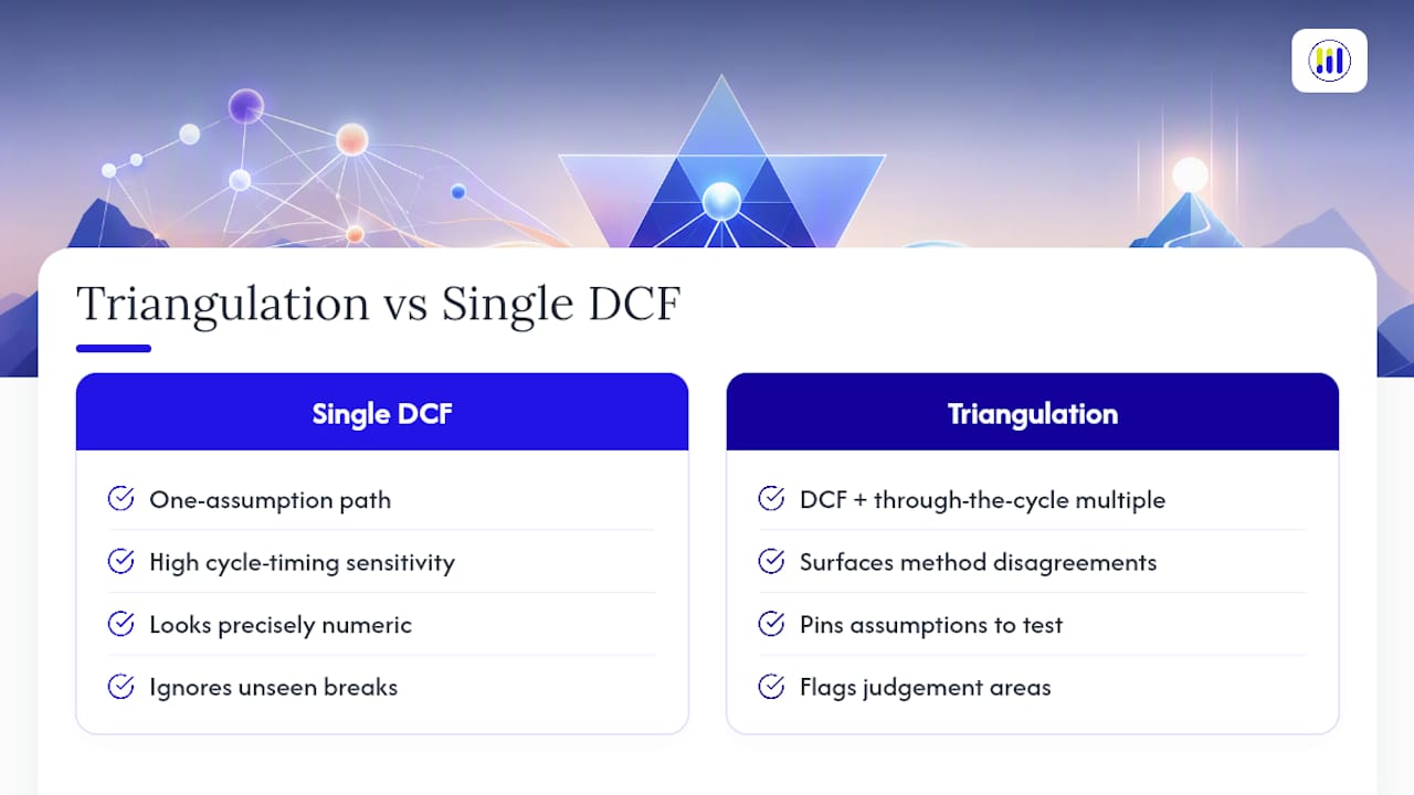
Why We Push Triangulation Over Any Single Model — overview diagram

Triangulating between a probability-weighted DCF and a through-the-cycle multiple does not eliminate uncertainty. It surfaces it. When the two methods converge, you have real conviction. When they diverge, that gap tells you exactly which assumption to interrogate before you commit capital, which is more useful than false precision from a single model.

The honest limitation is data. Structural breaks, a competitor's new low-cost plant, a permanent demand shift, do not show up cleanly in a historical margin series, and no calculator can flag a break that has not happened yet. That is a judgment call the model can inform but never replace. Tickerplace's coverage of over 10,000 US and ASX-listed companies, updated daily, exists to make the mechanical half of this workflow, pulling historical margins, running the multiples, weighting the scenarios, fast enough that you can spend your time on the judgment calls that actually separate a good cyclical call from a lucky one.

— Tickerplace

Put This Workflow to Work on a Real Cyclical Stock

Reading about normalization is one thing. Running it on an actual ticker in under ten minutes is another, and that gap is exactly what Tickerplace's free calculators are built to close for individual investors who don't have a Bloomberg terminal or a team of analysts behind them.

Start with a company's historical financials to pull the margin and capex history you need to build a mid-cycle baseline, then run that normalized figure through the intrinsic value calculator to generate a probability-weighted DCF instead of a single fragile point estimate. Cross-check the result against the EV/EBITDA calculator to see whether your DCF output and your through-the-cycle multiple actually agree. Every one of these tools is free, covers thousands of US and ASX-listed names, and updates daily, so the valuation band you build reflects current prices, not last quarter's snapshot. If you are stress-testing an entry point, the stock valuation checker gives you a fast read on whether the current price already sits inside or outside your band. Run your first normalized valuation today and see where the current price actually falls relative to the range.

Sources

The core prescription in this piece, normalize first, then triangulate, draws on a small set of sources worth reading directly if you want the underlying reasoning in full.

Aswath Damodaran's paper on valuing cyclical and commodity companies is the foundational text on why normalization beats cycle-timing, written by the valuation professor most cited on this exact problem. McKinsey's piece on valuing cyclical companies lays out the probabilistic, multi-scenario approach referenced throughout the scenario-DCF section. The ResearchGate study on market multiples provides the academic backing for averaging and robust multiple calculation. Model Reef's practitioner guide and AhaSignals' framework both translate the theory into the step-by-step mechanics used in the implementation workflow above, including the balance-sheet survival test.

FAQ

What Are the Four Main Types of Business Valuation?

The four core approaches are asset-based valuation, earnings-multiple valuation (comparable company analysis), discounted cash flow valuation, and market-based valuation using recent transaction data. For cyclical companies specifically, earnings-multiple and DCF approaches both require normalization before they produce reliable results.

What Does It Mean If a Company Is Cyclical?

A cyclical company's revenue and earnings rise and fall with the broader economy or with a specific commodity price, driven by shifts in volume, price, capacity utilization, and input costs. Airlines, homebuilders, steel producers, and miners are classic examples, distinct from defensive sectors like utilities or consumer staples whose demand stays comparatively stable through a downturn.

What Is the Rule of 20 for Valuing Stocks?

The Rule of 20 is a rough heuristic stating that a fair P/E ratio equals 20 minus the current inflation rate, so a market P/E above that threshold suggests overvaluation and below it suggests undervaluation. It is a broad market-level rule of thumb, not a substitute for normalized, company-specific analysis, and it holds up poorly for individual cyclical stocks whose earnings themselves are unstable.

What Are Examples of Cyclical Stocks?

Common cyclical categories include steel and industrial metals producers, homebuilders, airlines, auto manufacturers, shipping and logistics companies, and oil and gas producers, since all of these see demand and pricing move with the broader economic cycle or a specific commodity price. The right valuation approach for any of them starts with normalizing earnings over a full cycle rather than relying on the most recent reported quarter.

How Do You Adjust the Discount Rate for a Cyclical Company?

Many practitioners add a modest premium to the discount rate for cyclical companies to reflect the added uncertainty in cash flow timing and amplitude, though this is a blunter tool than scenario weighting. A probability-weighted scenario DCF, which captures uncertainty explicitly in the cash flows themselves, is generally a more precise approach than trying to encode all of that uncertainty into a single discount rate adjustment.